lcurve (Single Series)In this example, we plot the light curve of a single time series from EXOSAT ME of the transient pulsar, EXO 2030+375. The light curve data is made of multiple files listed in all.txt: d63924.lc.Z d63934.lc.Z d63945.lc.Z d63954.lc.Z d63968.lc.Z d63980.lc.Z Executing the lcurve task (Screen output is in a fixed width font, while commentary is italicized): lcurve 1.0 (xronos5.18) Number of time series for this task[1] Ser. 1 filename +options (or @file of filenames +options)[file1] @all.txt We enter the filelist beginning with an `@` symbol, and lcurve reads in the files listed in all.txt
 Series 1 file   1:d63924.lc.Z

 Selected FITS extensions: 1 - RATE TABLE;

 Source ............ EXO2030+40          Start Time (d) ....  6368 11:36:56.100
 FITS Extension ....  1 - `RATE      `   Stop Time (d) .....  6368 14:28:08.127
 No. of Rows .......          342        Bin Time (s) ......    30.00
 Right Ascension ... 307.624755960       Internal time sys.. Converted to TJD
 Declination ....... 37.416656430        Experiment ........ EXOSAT   ME

 Corrections applied: Vignetting - Yes; Deadtime - Yes; Bkgd - Yes; Clock - No
             values: .964785340       .911577050       1.00000000

 Selected Columns:  1- Y-axis;  2- Y-error;

 File contains binned data.

 Series 1 file   2:d63934.lc.Z

 Selected FITS extensions: 1 - RATE TABLE;

 Source ............ EXO2030+40          Start Time (d) ....  6368 14:44:12.129
 FITS Extension ....  1 - `RATE      `   Stop Time (d) .....  6368 18:24:28.162
 No. of Rows .......          440        Bin Time (s) ......    30.00
 Right Ascension ... 307.624755960       Internal time sys.. Converted to TJD
 Declination ....... 37.416656430        Experiment ........ EXOSAT   ME

 Corrections applied: Vignetting - Yes; Deadtime - Yes; Bkgd - Yes; Clock - No
             values: .983090820       .909090880       1.00000000

 Selected Columns:  1- Y-axis;  2- Y-error;

 File contains binned data.

 Series 1 file   3:d63945.lc.Z

 Selected FITS extensions: 1 - RATE TABLE;

 Source ............ EXO2030+40          Start Time (d) ....  6368 18:38:52.164
 FITS Extension ....  1 - `RATE      `   Stop Time (d) .....  6368 21:16:44.185
 No. of Rows .......          315        Bin Time (s) ......    30.00
 Right Ascension ... 307.624755960       Internal time sys.. Converted to TJD
 Declination ....... 37.416656430        Experiment ........ EXOSAT   ME

 Corrections applied: Vignetting - Yes; Deadtime - Yes; Bkgd - Yes; Clock - No
             values: .964785340       .910746750       1.00000000

 Selected Columns:  1- Y-axis;  2- Y-error;

 File contains binned data.

 Series 1 file   4:d63954.lc.Z

 Selected FITS extensions: 1 - RATE TABLE;

 Source ............ EXO2030+40          Start Time (d) ....  6368 21:32:12.186
 FITS Extension ....  1 - `RATE      `   Stop Time (d) .....  6369 01:48:04.208
 No. of Rows .......          511        Bin Time (s) ......    30.00
 Right Ascension ... 307.624755960       Internal time sys.. Converted to TJD
 Declination ....... 37.416656430        Experiment ........ EXOSAT   ME

 Corrections applied: Vignetting - Yes; Deadtime - Yes; Bkgd - Yes; Clock - No
             values: .983090820       .909918130       1.00000000

 Selected Columns:  1- Y-axis;  2- Y-error;

 File contains binned data.

 Series 1 file   5:d63968.lc.Z

 Selected FITS extensions: 1 - RATE TABLE;

 Source ............ EXO2030+40          Start Time (d) ....  6369 02:05:24.209
 FITS Extension ....  1 - `RATE      `   Stop Time (d) .....  6369 05:47:16.215
 No. of Rows .......          443        Bin Time (s) ......    30.00
 Right Ascension ... 307.624755960       Internal time sys.. Converted to TJD
 Declination ....... 37.416656430        Experiment ........ EXOSAT   ME

 Corrections applied: Vignetting - Yes; Deadtime - Yes; Bkgd - Yes; Clock - No
             values: .945537030       .911577050       1.00000000

 Selected Columns:  1- Y-axis;  2- Y-error;

 File contains binned data.

 Series 1 file   6:d63980.lc.Z

 Selected FITS extensions: 1 - RATE TABLE;

 Source ............ EXO2030+40          Start Time (d) ....  6369 06:03:00.215
 FITS Extension ....  1 - `RATE      `   Stop Time (d) .....  6369 10:18:36.212
 No. of Rows .......          510        Bin Time (s) ......    30.00
 Right Ascension ... 307.624755960       Internal time sys.. Converted to TJD
 Declination ....... 37.416656430        Experiment ........ EXOSAT   ME

 Corrections applied: Vignetting - Yes; Deadtime - Yes; Bkgd - Yes; Clock - No
             values: .983090820       .909918130       1.00000000

 Selected Columns:  1- Y-axis;  2- Y-error;

 File contains binned data.

Name of the window file ('-' for default window)[-]
Entering a - indicates that the default exposure windows are to be applied ($XRDEFAULTS/default_win.wi). A custom windows file may be generated with the xronwin task.
 Expected Start ...  6368.48398263830  (days)      11:36:56:100  (h:m:s:ms)
 Expected Stop ....  6369.42958578854  (days)      10:18:36:212  (h:m:s:ms)

 Minimum Newbin Time    30.000000      (s)
 for Maximum Newbin No..             2724

 Default Newbin Time is:   159.75775    (s) (to have 1 Intv. of     512 Newbins)
 Type INDEF to accept the default value

Newbin Time or negative rebinning[4.6692607009327] 200
Entering INDEF would divide the total timespan of the data into 512 equal newbins. Note: the number 512 may be modified with the hidden parameter, nbdf. You may not enter a newbin value less than the Minimum Newbin Time, which corresponds to the largest bin size found in the input files. In this example, we choose a newbin time of 200.
 Newbin Time ......     200.00000      (s)
 Maximum Newbin No.               409

 Default Newbins per Interval are:         409
 (giving       1 Interval of          409 Newbins)
 Type INDEF to accept the default value

Number of Newbins/Interval[10] indef
Entering INDEF includes the whole timespan of the input in the resulting plot. In order to subdivide the time series into multiple intervals, resulting in multiple plots, give a smaller number than the indicated INDEF value.
 Maximum of       1 Intvs. with          409 Newbins of       200.000     (s)
Name of output file[default]
In this example, we enter a space before pressing Return to indicate that an output FITS file is not desired, however, entering default for the output file, will result in a binned FITS light curve file to be written with the extension .flc. Note: In cases using a filelist, entering a specific filename rather than default is recommended, as the default output file uses only the first file in the list to construct the file name.
Do you want to plot your results?[yes] In general, we want to plot the binned light curve, however, entering no will prevent lcurve from plotting the output. This is useful when only the output FITS file is desired.
Enter PGPLOT device[/XW] The Xwindows device, /xw is recommended as the results may be viewed immediately and the plot may be manipulated interactively with PLT. In some cases, however, other file-based devices such as /ps and /gif may be desired.
     409 analysis results per interval


 Intv    1   Start  6368 11:38:21
     Ser.1     Avg  53.04        Chisq 0.6966E+06   Var  1026.     Newbs.    390
               Min  23.93          Max  153.7    expVar 0.5855      Bins   2559
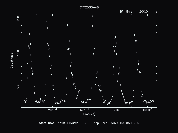
By default, the following plot is produced:
It may, however, by manipulated with any PLT command.
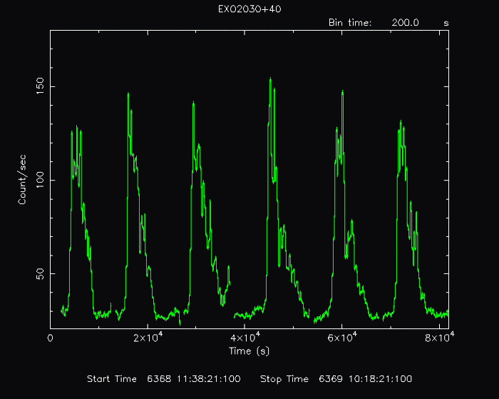
PLT> line step Connect the points.
PLT> color 3 on 2 Change group 2 (the data representing Y) to color 3 (green).
PLT> r x 0 82000 Rescale the x-axis from 0 to 82000.
PLT> r y,,180 Rescale the y-axis from the current minimum value to 180.
PLT> cpd exo2030_375.gif/gif Change the plot device to a gif.
PLT> p Plot to the gif.
PLT> quit The resulting gif file looks like this:
Note: If a particular sequence of commands is to be used multiple times, using a plot file may save some time. Rather than entering PLT commands interactively, a script file containing the commands usually with the extension .pco can be given for the hidden parameter, plotfile. For example, we can place the interactive commands used above into the file lcurve.pco: line step color 3 on 2 r x 0 82000 cpd exo2030_375.gif/gif p quitIf lcurve is executed like this: > lcurve plotfile=lcurve.pcoThe program will execute the commands, creating the exo2030_375.gif graphic and exiting the program automatically with no interaction at the PLT prompt. This is a useful option for automated plot generation provided all the required parameters are set when the task is executed.
Please send reports of errors to : xanprob@athena.gsfc.nasa.gov HEASARC Home | Observatories | Archive | Calibration | Software | Tools | Students/Teachers/Public Last modified: Friday, 26-Mar-2004 16:35:04 EST |


