lcurve (2 Series)
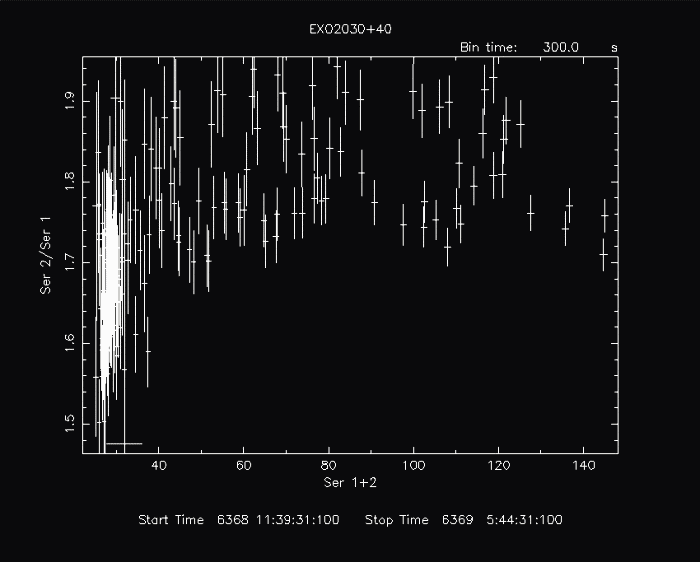
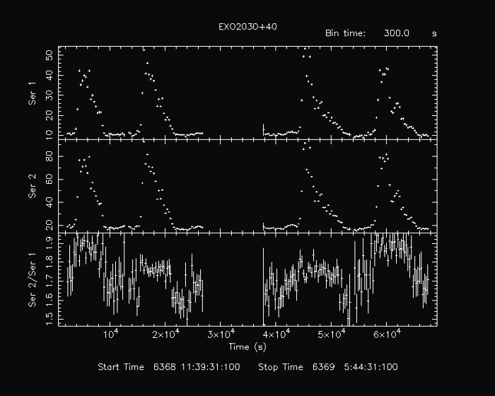
Enter multiples files for each time series Multiple files for each time series can be entered using an ascii file containing the list of input filenames. This list has the following format: filenames of the individual lightcurve or event file are listed one per line and the group of files that belong to different time series are separated by three slashes. In this example lcurve is run with two time series, each with four files, so the input file list, filelist.txt, looks like the following: me_a63924.lc me_a63934.lc me_a63954.lc me_a63968.lc /// me_b63924.lc me_b63934.lc me_b63954.lc me_b63968.lc Running lcurve to create light curve and hardness ratio plots The example uses the file list created above. The output lightcurve is binned with 300 seconds and data are organized in an interval with 219 points. When run with 2 time series lcurve calculates the hardness ratio. The three 300 sec bin time series, the hardness ratio and the sum of both time series are assembled in one array and passed to "PLT >" for plotting. By default lcurve prepares a plot based on the input to: Three plotting styles available: Hardness [1] ; Intensity vs Time (or Phase) [2]; Ratio & Intensity vs time (or Phase)[3] Enter PLOT style number (default=1)[3] 1however since all the calculated data are available in "PLT >" , any other plot (e.g. hardness vs time) can be obtained by using within "PLT >" the commands to turn on-off arrays.
lcurve 1.0 (xronos5.18)
Number of time series for this task[1] 2
Ser. 1 filename +options (or @file of filenames +options)[@filelist.txt]
Series 1 file 1:me_a63924.lc
Selected FITS extensions: 1 - RATE TABLE;
Source ............ EXO2030+40 Start Time (d) .... 6368 11:37:01.600
FITS Extension .... 1 - `RATE ` Stop Time (d) ..... 6368 14:28:13.627
No. of Rows ....... 10265 Bin Time (s) ...... 1.000
Right Ascension ... 307.624755960 Internal time sys.. Converted to TJD
Declination ....... 37.416656430 Experiment ........ EXOSAT ME
Corrections applied: Vignetting - Yes; Deadtime - Yes; Bkgd - Yes; Clock - No
values: .964785340 .911577050 1.00000000
Selected Columns: 1- Y-axis; 2- Y-error;
File contains binned data.
Series 1 file 2:me_a63934.lc
Selected FITS extensions: 1 - RATE TABLE;
Source ............ EXO2030+40 Start Time (d) .... 6368 14:43:57.629
FITS Extension .... 1 - `RATE ` Stop Time (d) ..... 6368 18:24:13.662
No. of Rows ....... 13209 Bin Time (s) ...... 1.000
Right Ascension ... 307.624755960 Internal time sys.. Converted to TJD
Declination ....... 37.416656430 Experiment ........ EXOSAT ME
Corrections applied: Vignetting - Yes; Deadtime - Yes; Bkgd - Yes; Clock - No
values: .983090820 .909090880 1.00000000
Selected Columns: 1- Y-axis; 2- Y-error;
File contains binned data.
Series 1 file 3:me_a63954.lc
Selected FITS extensions: 1 - RATE TABLE;
Source ............ EXO2030+40 Start Time (d) .... 6368 21:31:57.686
FITS Extension .... 1 - `RATE ` Stop Time (d) ..... 6369 01:47:49.708
No. of Rows ....... 15345 Bin Time (s) ...... 1.000
Right Ascension ... 307.624755960 Internal time sys.. Converted to TJD
Declination ....... 37.416656430 Experiment ........ EXOSAT ME
Corrections applied: Vignetting - Yes; Deadtime - Yes; Bkgd - Yes; Clock - No
values: .983090820 .909918130 1.00000000
Selected Columns: 1- Y-axis; 2- Y-error;
File contains binned data.
Series 1 file 4:me_a63968.lc
Selected FITS extensions: 1 - RATE TABLE;
Source ............ EXO2030+40 Start Time (d) .... 6369 02:05:09.709
FITS Extension .... 1 - `RATE ` Stop Time (d) ..... 6369 05:47:01.715
No. of Rows ....... 13305 Bin Time (s) ...... 1.000
Right Ascension ... 307.624755960 Internal time sys.. Converted to TJD
Declination ....... 37.416656430 Experiment ........ EXOSAT ME
Corrections applied: Vignetting - Yes; Deadtime - Yes; Bkgd - Yes; Clock - No
values: .945537030 .911577050 1.00000000
Selected Columns: 1- Y-axis; 2- Y-error;
File contains binned data.
Series 2 file 1:me_b63924.lc
Selected FITS extensions: 1 - RATE TABLE;
Source ............ EXO2030+40 Start Time (d) .... 6368 11:37:01.600
FITS Extension .... 1 - `RATE ` Stop Time (d) ..... 6368 14:28:13.627
No. of Rows ....... 10265 Bin Time (s) ...... 1.000
Right Ascension ... 307.624755960 Internal time sys.. Converted to TJD
Declination ....... 37.416656430 Experiment ........ EXOSAT ME
Corrections applied: Vignetting - Yes; Deadtime - Yes; Bkgd - Yes; Clock - No
values: .964785340 .911577050 1.00000000
Selected Columns: 1- Y-axis; 2- Y-error;
File contains binned data.
Series 2 file 2:me_b63934.lc
Selected FITS extensions: 1 - RATE TABLE;
Source ............ EXO2030+40 Start Time (d) .... 6368 14:43:57.629
FITS Extension .... 1 - `RATE ` Stop Time (d) ..... 6368 18:24:13.662
No. of Rows ....... 13209 Bin Time (s) ...... 1.000
Right Ascension ... 307.624755960 Internal time sys.. Converted to TJD
Declination ....... 37.416656430 Experiment ........ EXOSAT ME
Corrections applied: Vignetting - Yes; Deadtime - Yes; Bkgd - Yes; Clock - No
values: .983090820 .909090880 1.00000000
Selected Columns: 1- Y-axis; 2- Y-error;
File contains binned data.
Series 2 file 3:me_b63954.lc
Selected FITS extensions: 1 - RATE TABLE;
Source ............ EXO2030+40 Start Time (d) .... 6368 21:31:57.686
FITS Extension .... 1 - `RATE ` Stop Time (d) ..... 6369 01:47:49.708
No. of Rows ....... 15345 Bin Time (s) ...... 1.000
Right Ascension ... 307.624755960 Internal time sys.. Converted to TJD
Declination ....... 37.416656430 Experiment ........ EXOSAT ME
Corrections applied: Vignetting - Yes; Deadtime - Yes; Bkgd - Yes; Clock - No
values: .983090820 .909918130 1.00000000
Selected Columns: 1- Y-axis; 2- Y-error;
File contains binned data.
Series 2 file 4:me_b63968.lc
Selected FITS extensions: 1 - RATE TABLE;
Source ............ EXO2030+40 Start Time (d) .... 6369 02:05:09.709
FITS Extension .... 1 - `RATE ` Stop Time (d) ..... 6369 05:47:01.715
No. of Rows ....... 13305 Bin Time (s) ...... 1.000
Right Ascension ... 307.624755960 Internal time sys.. Converted to TJD
Declination ....... 37.416656430 Experiment ........ EXOSAT ME
Corrections applied: Vignetting - Yes; Deadtime - Yes; Bkgd - Yes; Clock - No
values: .945537030 .911577050 1.00000000
Selected Columns: 1- Y-axis; 2- Y-error;
File contains binned data.
Name of the window file ('-' for default window)[-]
Expected Start ... 6368.48404629571 (days) 11:37: 1:600 (h:m:s:ms)
Expected Stop .... 6369.24099207078 (days) 5:47: 1:715 (h:m:s:ms)
Minimum Newbin Time 1.0000000 (s)
for Maximum Newbin No.. 65401
Default Newbin Time is: 127.88446 (s) (to have 1 Intv. of 512 Newbins)
Type INDEF to accept the default value
Newbin Time or negative rebinning[300]
Newbin Time ...... 300.00000 (s)
Maximum Newbin No. 219
Default Newbins per Interval are: 219
(giving 1 Interval of 219 Newbins)
Type INDEF to accept the default value
Number of Newbins/Interval[219]
Maximum of 1 Intvs. with 219 Newbins of 300.000 (s)
Name of output file[]
Do you want to plot your results?[yes]
Enter PGPLOT device[/XW]
Setting the plot to 1 "PLT >" plots the hardness ratio vs. the sum of the light curves; setting the plot type to 2 (= number of time series) "PLT >" the light curves (intensity vs. time) on separate windows; setting the plot type to 3 "PLT >" plots the light curves for series 1 and 2 followed by the hardness ratio vs. time in separate windows. After the default plot is done, within "PLT >" is possible to plot any axis vs any other by using the command "color on" or "color off" and "xaxis N" or "yplot M".
 Three plotting styles available:
 Hardness [1] ;  Intensity vs Time (or Phase) [2];
 Ratio & Intensity vs time (or Phase)[3]
Enter PLOT style number (default=1)[3] 1
219 analysis results per interval
Intv 1 Start 6368 11:39:31
Ser.1 Avg 18.72 Chisq 0.1161E+06 Var 124.1 Newbs. 178
Min 9.094 Max 53.43 expVar 0.1983 Bins 51868
Ser.2 Avg 33.13 Chisq 0.2765E+06 Var 429.5 Newbs. 178
Min 15.30 Max 92.51 expVar 0.2874 Bins 51868
PLT>

If the Intensity vs. Time plot type (2 in this case) had been chosen, the following plot would result: 
If the Ratio and Intensity vs. Time plot type (i.e. 3) had been chosen, the following plot would result: 
It is possible to use the PLT prompt to customize
the output plot.
The command "info" lists all the columns available which are:
At the PLT> prompt you will be able to use any of the "QDP" commands
documented in the
qdp help file.
HEASARC Home | Observatories | Archive | Calibration | Software | Tools | Students/Teachers/Public Last modified: Friday, 26-Mar-2004 16:35:03 EST |

